


Most of the constructive feedback I received about this article was “Nice explanation, but your pipeline is 6 years old!”. I wasn’t sure what that exactly meant until Christoph Kubisch joined my fight in the Render Hell. He is a Developer Technology Engineer working for NVIDIA and whatever question I had, he answered it. And believe me, I had a lot! :)
Be aware that we omitted and simplified some details.
Two major points of the pipeline will be explained below, which weren’t totally wrong explained here in book I, but might not be clear enough:
2. There can be several parallel running pipelines!
Below I’ll go into detail about it. Have fun!
1. Not everything is done by the “tiny” GPU cores!
In the pipeline example above it might seem like every pipeline stage is done by the GPU Cores – This is NOT the case! In fact, most of the stuff is not done by them. In the new section in “1. Copy the data into system memory for fast access” you already saw that several components are necessary to just bring the data to a core. So what work do the cores actually do?
Let’s observe one:
A core can receive commands and data. Then it executes the command by calculating the data in a floating point unit (FP UNIT) or an integer unit (INT UNIT). So you could say: A core can calculate pixels and vertices (maybe also other calculations like physics but let’s focus on graphic rendering).
Other important stuff like distribute the render-tasks, calculate tessellation, culling and preparing the fragments for the pixel shader, depth testing and writing pixels into the frame buffer are NOT done by the cores. This work is done by special, not programmable hardware blocks which are also placed in the GPU.
Ok, after we know that now, let’s move on to the next major point I have to clear out:
2. There can be several parallel running pipelines!
First, I’ll give you a short example what I mean with that headline. If you’re still thirsty after this, I’ll take you into an even more detailed explanation.
But first, let’s recap:
If we would only have one GPU Core, what could we calculate with it?

Correct: Nothing! Because the core needs someone who assigns him some work. This is done by a Streaming Multiprocessor which can handle a stream of vertices/pixels which belong to one shader. OK, with that and one core we could calculate one vertex/pixel at a time:

Of course, if we increase the amount of cores, there can be more vertices/pixels calculated at the same time. But only if they belong to the same shader!

This was already explained in my first attempt of explaining the pipeline! But now it gets interesting: What if we would add another Streaming Multiprocessor which cares about half of the cores?

Now we can not only calculate vertices/pixels in parallel, we can also take care about 2 shader streams at the same time! This means, we can for example run two different pixel shaders at the same time or run a vertex shader AND a pixel shader at the same time!
This rough example shall just give you a glimpse about that several different hardware blocks are involved and they all work in parallel so the pipeline is more flexible than I described in my first attempt.
Anyone still thirsty? Then let’s get into more detail!
3. In-Depth look into the pipeline stages
3.1 Overview
First of all: Why do we need a flexible/parallel pipeline? The reason is, that you can’t foresee, what workload you’ll have. Especially with tessellation it might be, that there are suddenly 100.000 more polygons on the screen than one frame before. Therefore you need a flexible pipeline which handles totally different workloads.
DON’T WORRY!
Please don’t be afraid by looking at the two following images (like I am when i read a Wikipedia article and see formulas between the text)! Yes, this stuff isn’t easy and even complex charts only show what a programmer needs to know and hide a lot of the “real” complexity. I only show it to give you a rough understand how complicated this stuff is. :)
The following image shows a GPU. I have no idea about what is what, but it’s kind of beautiful, isn’t it?
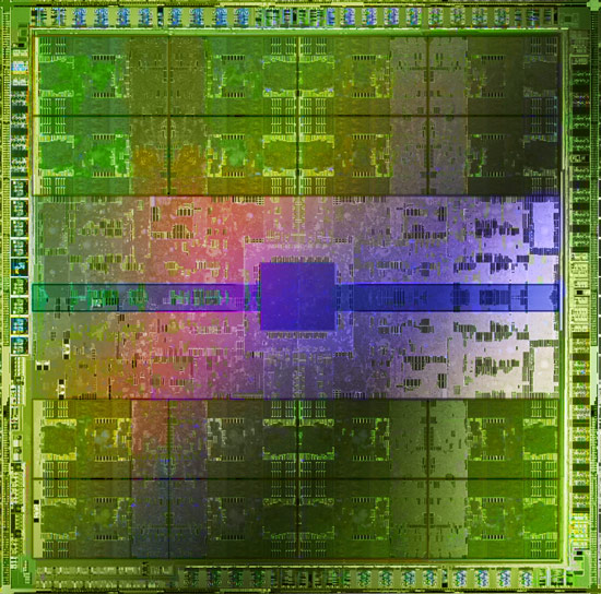
Source: http://www.legitreviews.com/
And here’s an image from Christoph Kubisch’ Article “Life of a triangle”. It shows parts of the work which is happening on a GPU in structured graphics.

I hope you’ve a rough idea about the complexity now and will realize how much the explanations below are simplified. Let’s now have a detailed look on the whole pipeline.
3.2 Application Stage
It starts with the application or a game telling the driver that it wants something rendered.
3.3 Driver Stage
The driver receives the commands from the application and puts them into a command buffer (this was already explained here in book I). After a while (or when the programmer forces it), the commands are send to the GPU.
3.4 Read commands
Now we’re on the graphic card! The Host Interface reads commands to make them available for further use.
3.5 Data Fetch
Some of the commands sent to the GPU can contain data or are instructions to copy data. The GPU typically has a dedicated engine to deal with copying data from RAM to VRAM and vice versa. This data could be anything filling vertex buffers, textures or other shader parameter buffers. Our frame would typically start with some camera matrices being sent.
- I symbolize the data as geometries but in fact we’re talking just about vertex-lists (vertex buffer). For a long time the rendering process doesn’t care about the final model. Instead, most of the time, only single vertices/pixels are worked with.
- Textures only get copied, if they’re not already in the VRAM on the graphic card!
- If vertex buffer are used a lot, they can stay in the VRAM like textures and don’t have to be copied with every draw call
- Vertex buffers may stay in the RAM (not VRAM) if they change a lot. Then the GPU can read the data directly from RAM to its Caches.
Now that all ingredients are ready the Gigathread Engine comes into play, it creates a thread for every vertex/pixel and bundles them into a package. NVIDIA calls such a package: Thread Block. Additional threads may also be created for vertices after tessellation or for geometry shaders (will be explained later). Thread blocks are then distributed to the Streaming Multiprocessors.
3.6 Vertex Fetch
A Streaming Multiprocessor is a collection of different hardware units and one of them is the Polymorph Engine. For the sake of simplicity I present them like separate guys. :) The Polymorph Engine gets the needed data and copies it into caches so cores can work faster. Why it is useful to copy data into caches was explained here in book I.
3.7 Shader Execution
The main purpose of the Streaming Multiprocessor is executing program code written by the application developer, also called shaders. There is multiple types of shaders but each kind can run on any of these Streaming Multiprocesors and they all follow the same execution logic.
The Streaming Multiprocessor now takes his big Thread Block which he received from the Gigathread Engine and separates it into smaller chunks of work. He splits the Thread Block into heaps of 32 Threads. Such a smaller heap is called: Warp. In total, a Maxwell Streaming Multiprocessor can “hold” 64 of such warps. In my example and Maxwell GPUs there are 32 dedicated cores to work on the 32 Threads.
One Warp is then taken to be worked on. At this point the hardware should have all necessary data loaded into the registers so that the cores can work with it. We simplify the illustration here a bit: Maxwell’s Streaming Processor for example has 4 warp schedulers, which each would let one warp work and manage a subset of the Streaming Multiprocessor’s warps.
The actual work begins now. The cores itself never see the whole shader-code but only one command of it at the time. They do their work and then the next command is given to them by the Streaming Multiprocessor. All cores execute the same command but on different data (vertices/pixels). It’s not possible that some cores work on command A and some on command B at the same time. This method is called lock-step.
This lock-step method gets important if you have an IF-statement in your shader code which executes either one code block or another.
This IF-Statement makes some of our cores execute the left code and some the right code. It can’t be done at the same time (like explained above). First one code-side would be executed and some cores would be “sleeping” and then the other side is executed afterwards. Kayvon explains this here at 43:58 “What about conditional execution?”.
In my example 16 pixels/vertices would be worked on but it’s of course possible to have IF-statements where only ONE pixel/vertex is calculated and the other 31 cores get masked out. The same applies to loops, if only one core has to stay in the loop long, all the others become idle. This phenomenon is also called “divergent threads” and should be minimized. Ideally all threads in the warp hit the same side of the IF-condition, because then we can entirely jump over the non-active side.
But why can the Streaming Processor hold 64 warps, when the cores can only work on very few at a time?? This is because sometimes you can’t progress because you have to wait for some data. For example we need to calculate the lighting with the normal from our normal map texture. Even if the normal was in the cache it takes a while to access it, and if it wasn’t it can take a good while. Pro’s call this Memory Stall and this is greatly explained by Kayvon. Instead of doing nothing, the current warp will just be exchanged with one, where the necessary data is ready for use:
The explanation above was a bit simplified. Modern GPU architecture doesn’t only allow a Streaming Processor working at one Warp at the time. Look for example at this image showing a Streaming Processor (SMM) based on Maxwell architecture: One Streaming Processor has access to four Warp schedulers, each controlling 32 Cores. This makes him able to work on four Warps completely parallel. The book keeping for the work state of multiple threads is kept independently and is reflected by how many Threads the SM can hold in parallel, as noted on top.
Since more than 4 Warps can run in parallel in Maxwell. Each warp scheduler can perform dual-issuing instruction in one clock clock to a warp, in this sense, every clock cycle we have up to 4 warps get their new instructions to work on (suppose at least 4 warps are ready by far). However, we also have instruction-level parallelism. That means when 4 warps are executing instructions (typically with 10-20 cycle latency), the next batch of 4 warps can accept new instructions in the next clock cycle. Therefore, it is possible to have more than 4 warps running in parallel if the resources are available. Actually, in one of the CUDA optimization video in GTC2013, more than 30 active warps are recommended to keep the pipeline fully occupied in a general case. You may want to revise the wording here to indicate that there will be multiple (more than 4) warps running in parallel, to avoid any potential confusion that people may think 4 scheduler could only hold 4 parallel warps.
– Guohui Wang

But what are our threads actually working on? For example a Vertex Shader!
3.8 Vertex Shader
The vertex shader takes care of one vertex and modifies it how the programmer wants. Unlike normal software (e.g. Mail-Program) where you run one instance of the program and hand over a lot data which get taken care of (e.g. handling all the Mails), you run one instance of a vertex shader program for every vertex which then runs in in one thread managed by the Streaming Multiprocessor.
Our vertex shader transforms vertices or its parameters (pos, color, uv) like you want:
Click here for Tessellation Until here we only saw single vertices. Sure, they came in a specific order send by a programmer but we treated them independently and not as a group. The following sections deal with steps that are only done when tessellation shaders are being used. The first of such steps creates patches from the individual vertices. That way it is possible to subdivide them and add geometric detail. How many vertices make a patch is defined by the programmer, the maximum is, guess what, 32 vertices. In OpenGL is this stage called Patch/Primitive Assembly and in DirectX only Patch Assembly (Primitive Assembly comes later). More detailled information about patch/primitive assembly can be found in [a57]. 3.10 Hull Shader The Hull shader takes all the vertices which belong to the just created patch and calculates a tessellation factor e.g. dependent on the distance to the camera. As the hardware can only tessellate three basic shapes (quad, triangle or a series of lines), the shader code also contains which shape is being used by the tessellator. As a result there is not just a single tessellation factor, but they are computed for each outer side and also a special “inner” side of the shape. To be able to create meaningful geometry later, the Hull Shader also computes the input values for the Domain Shader, which takes care of the positions. 3.11 Tessellation Now we know in which shape and how much we want to subdivide the patch – the Polymorph Engine takes this information and does the actual work. Out of this arrive a lot new vertices. These are sent back to the Gigathread Engine to be distributed across the GPU and are handled by the Domain Shader. More information about the shader stages can be found here [a55] and here [a79]. Here you can find Detailed articles about Triangle Tesselation and Quad Tesselation. You might ask why not directly put the geometry detail into the model. There are two reasons for this. First, you might remember how accessing memory is slow compared to just doing calculations. So instead of having to fetch all those additional vertices with all their attributes (position, normal, uv…), it is better to generate them from less data (patch corner vertices + displacement logic or textures, which support mipmaps, compression…). Second, with tessellation you’re able to adjust the detail depending on the distance to the camera – so you’re very flexible. Otherwise we may compute tons of vertices, that belong to triangles that are not even visible in the end (too small or not in view). 3.12 Domain Shader Now the final position for the generated tessellation vertices are calculated. If the programmer wanted to use a displacement map, it is applied here. The input of the Domain Shader are the outputs of the Hull Shader (for example the patch vertices) as well as a barycentric coordinate from the tessellator. With the coordinate and the patch vertices you can compute a new position of the vertex, and you can then apply the displacement to it. Similar to a vertex shader, the Domain Shader computes the data passed to the next shader stages, which can be either the Geometry Shader if active, or the Fragment Shader. 3.13 Primitive Assembly Towards the end of the geometry pipeline we gather the vertices that assemble our primitive: a triangle, line or point. The vertices either came from the vertex shader, or if tessellation was active from the domain shader. What mode (triangle, line or point) we are in was defined in the application for this drawcall. Normally we would just pass the primitive for final processing and rasterzation, but there is an optional stage that makes use of this information, the Geometry Shader. 3.14 Geometry Shader The Geometry Shader works on the final primitives. Similar to the Hull Shader it gets the primitive’s vertices as input. It can modify those vertices and even generate a few new ones. It can also change the actual primitive mode. For example turn a point into two triangles, or the three visible sides of a cube. However it is not really good for creating lots of new vertices or triangles, tessellation is best left to the tessellation shaders. Its purpose is rather special given it’s the last stage prior preparing the primitive for rasterization. For example it plays a key-role in current voxelization techniques. Here you can find good examples how to program & use geometry shaders. And this is a great overview about the openGL pipeline. 3.15 Viewport Transform & Clipping Until here the programmers seem to use a quadratic space for all the operations (i guess it’s easier/faster that way) but now this needs to be fit to the actual resolution of your monitor (or window where the game is rendered into). More info about this you can find here in the “Viewport Transform / Screen Mapping” Section. Also triangles get cut if they overlap a certain security-border (Guard Band) of the scene (this is called: Guard Band Clipping and you find more infos here and here). The clipping is done because the Rastizer can only deal with triangles within the area it’s working on: 3.16 Triangles Journey This is not really a separate step in the pipeline but I found it very interesting so that it gets its own section. At this point we know the exact position, shading, etc. of several vertices which form triangles. These triangles need to be “painted” and before we can do that, someone has to find out which pixels of the screen are covered by the triangles. This is done by so called rasterizers. It’s important to know, that there are several available AND several of them can work at the same triangle if its big enough. Else it would mean that only one rasterizer is working when you have big triangles on screen and the others would have some vacation. Therefore every rasterizer has the responsibility for certain parts of the screen. And if a triangle belongs to such a responsibility area (the bounding box of the triangle is taken to measure this), it is send to this rasterizer so that he can work on it. 3.17 Rasterizing The rasterizer receives the triangles he’s responsible for and first does a quick check if the triangle even faces forward. If not, it’s thrown away (backface culling). If the triangle is “valid”, the rasterizer creates pre-pixels/fragments by calculating the edges which connect the vertices (edge setup) and so seeing which pixels quads (2×2 pixels) belong to the triangle. If you’re really into rasterizing and micro-triangles, you definitely should check out this presentation. And this article gives a good overview about it. After the pre-pixels/fragments are created, there’s a check if they would be even visible (or hidden by already rendered stuff):
Pixels produced by the rasterizer are sent to the Z-cull unit. The Z-cull unit takes a pixel tile and compares the depth of pixels in the tile with existing pixels in the framebuffer. Pixel tiles that lie entirely behind framebuffer pixels are culled from the pipeline, eliminating the need for further pixel shading work. 3.18 Pixel Shader After the pre-pixels/fragments are generated they can be “filled”. For every pre-pixel/fragment a new thread is generated and again distributed to all the available cores (like it was done with all the vertices). “Again we batch up 32 pixel threads, or better say 8 times 2×2 pixel quads, which is the smallest unit we will always work with in pixel shaders.” When the cores are done with their work, they write the results into the registers from where they are taken and put into the caches for the last step: Raster Output (ROP). 3.19 Raster Output The final step is done by the so called “Raster Output” Units which move the final pixel data (just got from the pixel shader) from L2 cache into the framebuffer which lays around in the VRAM. The GF100 as an example has 48 such ROPs and I interpret the dataflow (from L2 cache to VRAM) based on that they are placed really near to each other:
“[…] L2 cache, and ROP group are closely coupled […]” Besides of just moving pixel data, the ROPs also take care of pixel blending, coverage information for anti aliasing and “atomic operations”. What a ride, it took a long time to bring all the information together so I hope you found this book useful. The End.
3.9 Patch Assembly
– NVIDIA GF100 Whitepaper
– NVIDIA GF 100 Whitepaper

Oh My God. This is brilliant! Please compile all this into a massive PDF!
I’m afraid a PDF isn’t really useful because the whole article lives from all the animation which can’t be displayed in a PDF. :( But if you have an idea how it would be possible, let me know! :)
WOW fast response!, I did realise after typing it, but i got too sucked into reading to actually correct it!.
Heres some errors i noticed (but very minor)
“Until here we only saw single vertices. Sure, they came in a specific order send by a programmer but we threated them independently and not as a group. The following ”
Should be “Treated”.
Also,
“L2 cache, and ROP group are closely”
– NVIDIA GF 100 Whitepaper
Is that quote correct because it doesn’t make much sense in english!
Either way, thank you so much for taking the time to make this! I’m not a programmer (I’ve written a simple engine but I’m amateur), I’m a 3D artist, but I really like to learn about this stuff to create my own tools and honestly, the renderhell series is like a bible! Please find a way to put them all into 1 big book, make “step-by-step drawings” to replace the animations and print a hard-copy. I’d buy it! You’re a fantastic teacher!
Thanks man! You make me blushed :) But don’t forget to thank Christoph, without him there would be no Pipeline Book. :) I corrected the mistakes, thanks a lot pointing them out! The quote now is “[…] “L2 cache, and ROP group are closely coupled […]” like it’s in the paper.
Wow great to hear that you’re an artist with technical tendency! It’s the same for me but I’m not able to write an engine – props to you! :) I guess then you’re in general also interesting in improving workflows and have structures which help to be more productive?
Great article! Thanks, Simon.
Want to report minor errors:
3.11 Tesselation “… can be found here [a55] and here [a58].” Second link doesn’t work because of a mistake in html attribute name (“hreaf” instead of “href”). And the link itself differs with a link in [a58] (here “http://www.hotchips.org/wp-content/uploads/hc_archives/hc22/HC22.23.110-1-Wittenbrink-Fermi-GF100.pdf” and in the book index [a58] points to “http://cg.informatik.uni-freiburg.de/course_notes/graphics_01_pipeline.pdf”)
Thanks a lot! I just fixed the mistakes :)
Hi, thanks for the really interesting and useful tutorial.
I want to point out one issue I found here “Look for example at this image showing a Streaming Processor (SMM) based on Maxwell architecture: One Streaming Processor has access to four Warp schedulers, each controlling 32 Cores. This makes him able to work on four Warps completely parallel.”
This is not very accurate, since more than 4 Warps can run in parallel in Maxwell. Each warp scheduler can perform dual-issuing instruction in one clock clock to a warp, in this sense, every clock cycle we have up to 4 warps get their new instructions to work on (suppose at least 4 warps are ready by far). However, we also have instruction-level parallelism. That means when 4 warps are executing instructions (typically with 10-20 cycle latency), the next batch of 4 warps can accept new instructions in the next clock cycle. Therefore, it is possible to have more than 4 warps running in parallel if the resources are available. Actually, in one of the CUDA optimization video in GTC2013, more than 30 active warps are recommended to keep the pipeline fully occupied in a general case. You may want to revise the wording here to indicate that there will be multiple (more than 4) warps running in parallel, to avoid any potential confusion that people may think 4 scheduler could only hold 4 parallel warps.
Thanks again for the brilliant article!
Thank you for the kind words and taking the time to write this comment! I’ve just added it to the article so that other people can see it more easily. :)
https://simonschreibt.de/gat/renderhell-book2/#update2-1
Hi Guohui,
Thanks for your explanation.
I’m here to just confirm my understanding about “That means when 4 warps are executing instructions (typically with 10-20 cycle latency), the next batch of 4 warps can accept new instructions in the next clock cycle”. Does it behave like pipelining in CPU. E.g., there are five stages for any one instruction (ideally), which are instruction fetching (IF), instruction decoding (ID), execution (EXE), memory access (MEM), writing back (WB). If at clock cycle (cc) 1 instruction A operates at the 2nd stage ID, there will be available resources which allow another instruction to run at stage IF. To take full advantage of the precious resources of a CPU, instruction B could operate at stage IF. Therefore at cc 1, there are two instructions running parallelly even they are at different stages.
Is my comprehension right? Thank you.
Hi Guohui, thanks for your explanation.
If you don’t mind, I just wanna confirm my understanding.
In my opinion, there are two kinds of strategies which can help instruction-level parallelism, multi-issuing and pipelining, which I learnt from CPU. Let’s consider only multi-issuing at first, given that 4 warps schedulers and “dual-issuing” for each scheduler, why aren’t there 8 warps operated in one clock cycle (cc), but 4 that you’ve mentioned? Then, we need to consider pipelining so the number of warps operated at one cc will keep increasing, right? I’m a bit confused.
Thanks a lot.
Or do you indicate 4 wraps are executed in one cc but 8 instructions could be parallel? Thank you.
Great Work! good job.
I’ve got many things from your article.
Thanks.
And I found an unavailable link.
Also triangles get cut if they overlap a certain security-border (Guard Band) of the scene (this is called: Guard Band Clipping and you find more infos here and here). The clipping is done because the Rastizer can only deal with triangles within the area it’s working on:
In this sentence, the first orange-colored link is not working.
Thanks! I’ll have a look on it :)
Hi, thanks for your fantastic article!
There is a tiny question because I’m a newbie just stepping into the brand new field.
“Maxwell’s Streaming Processor for example has 4 warp schedulers, which each would let one warp work and manage a subset of the Streaming Multiprocessor’s warps”, and we also know “He splits the Thread Block into heaps of 32 Threads. Such a smaller heap is called: Warp”. Does it mean that a Maxwell’s Streaming Multiprocessor can couple 4 * 32 = 128 threads?
But meanwhile, “In my example and Maxwell GPUs there are 32 dedicated cores to work on the 32 Threads”. There are just 32 threads, how do they couple with 128 threads?
Looking forward your reply!
Sorry for my misunderstanding.
After reading the spec of Maxwell, I’ve clarified that each Maxwell’s Streaming Processor has 4 Warp Schedulers. And each warp scheduler has 32 threads, so there are 4 * 32 = 128 threads that can be executed parallelly in total without the consideration of instruction-level parallelism like multi-issuing and pipelining.
Hi Simon!
Thank you for all the hard work and dedication!
I’ve just noticed that this picture is not loading on the page: (http://ck.luxinia.de/blog/fermipipeline.png)
“Source: Christoph Kubisch’ Article “Life of a triangle””.
Just so you know.
Thank you for the report, I will have a look!